Section 5 Sentiment Analysis
This part of the workshop showcases how to perform SA on textual data using R. The analysis shown here is in parts based on the 2nd chapter of Text Mining with R - the e-version of this chapter on sentiment analysis can be found here.
SENTIMENT-ANALYSIS TOOL
You can also check out the free, online, notebook-based, R-based Sentiment-Analysis Tool offered by LADAL.
5.1 What is Sentiment Analysis?
Sentiment Analysis (SA) extracts information on emotion or opinion from natural language (Silge and Robinson 2017). Most forms of SA provides information about positive or negative polarity, e.g. whether a tweet is positive or negative. As such, SA represents a type of classifier that assigns values to texts. As most SA only provide information about polarity, SA is often regarded as rather coarse-grained and, thus, rather irrelevant for the types of research questions in linguistics.
In the language sciences, SA can also be a very helpful tool if the type of SA provides more fine-grained information. In the following, we will perform such a information-rich SA. The SA used here does not only provide information about polarity but it will also provide association values for eight core emotions.
The more fine-grained output is made possible by relying on the Word-Emotion Association Lexicon (Mohammad and Turney 2013), which comprises 10,170 terms, and in which lexical elements are assigned scores based on ratings gathered through the crowd-sourced Amazon Mechanical Turk service. For the Word-Emotion Association Lexicon raters were asked whether a given word was associated with one of eight emotions. The resulting associations between terms and emotions are based on 38,726 ratings from 2,216 raters who answered a sequence of questions for each word which were then fed into the emotion association rating (cf. Mohammad and Turney 2013). Each term was rated 5 times. For 85 percent of words, at least 4 raters provided identical ratings. For instance, the word cry or tragedy are more readily associated with SADNESS while words such as happy or beautiful are indicative of JOY and words like fit or burst may indicate ANGER. This means that the SA here allows us to investigate the expression of certain core emotions rather than merely classifying statements along the lines of a crude positive-negative distinction.
We start by writing a function that clean the data. This allows us to feed our texts into the function and avoids duplicating code. Also, this showcases how you can write functions.
# Define a function 'txtclean' that takes an input 'x' and a 'title'
txtclean <- function(x, title) {
  # Load required libraries
  require(dplyr)
  require(stringr)
  require(tibble)
  # Convert encoding to UTF-8
  x <- x %>%
    iconv(to = "UTF-8") %>%
    # Convert text to lowercase
    base::tolower() %>%
    # Collapse text into a single string
    paste0(collapse = " ") %>%
    # Remove extra whitespace
    stringr::str_squish() %>%
    # Split text into individual words
    stringr::str_split(" ") %>%
    # Unlist the words into a vector
    unlist() %>%
    # Convert the vector to a tibble
    tibble::tibble() %>%
    # Select the first column and name it 'word'
    dplyr::select(word = 1, everything()) %>%
    # Add a new column 'type' with the given title
    dplyr::mutate(type = title) %>%
    # Remove stop words
    dplyr::anti_join(stop_words) %>%
    # Remove non-word characters from the 'word' column
    dplyr::mutate(word = str_remove_all(word, "\\W")) %>%
    # Filter out empty words
    dplyr::filter(word != "")
}
Process and clean texts.
# process text data
posreviews_clean <- txtclean(posreviews, "Positive Review")
negreviews_clean <- txtclean(negreviews, "Negative Review")
# inspect
str(posreviews_clean); str(negreviews_clean)
## tibble [95,527 × 2] (S3: tbl_df/tbl/data.frame)
## $ word: chr [1:95527] "reviewers" "mentioned" "watching" "1" ...
## $ type: chr [1:95527] "Positive Review" "Positive Review" "Positive Review" "Positive Review" ...## tibble [90,656 × 2] (S3: tbl_df/tbl/data.frame)
## $ word: chr [1:90656] "basically" "family" "boy" "jake" ...
## $ type: chr [1:90656] "Negative Review" "Negative Review" "Negative Review" "Negative Review" ...Now, we combine the data with the Word-Emotion Association Lexicon (Mohammad and Turney 2013).
# Combine positive and negative reviews into one dataframe
reviews_annotated <- rbind(posreviews_clean, negreviews_clean) %>%
  # Group the combined dataframe by the 'type' column
  dplyr::group_by(type) %>%
  # Add a new column 'words' with the count of words for each group
  dplyr::mutate(words = n()) %>%
  # Join the sentiment data from the 'nrc' sentiment lexicon
  dplyr::left_join(tidytext::get_sentiments("nrc")) %>%
  # Convert 'type' and 'sentiment' columns to factors
  dplyr::mutate(type = factor(type),
                sentiment = factor(sentiment))

# inspect data
reviews_annotated %>%
  as.data.frame() %>%
  head(10)
## word type words sentiment
## 1 reviewers Positive Review 95527 <NA>
## 2 mentioned Positive Review 95527 <NA>
## 3 watching Positive Review 95527 <NA>
## 4 1 Positive Review 95527 <NA>
## 5 oz Positive Review 95527 <NA>
## 6 episode Positive Review 95527 <NA>
## 7 hooked Positive Review 95527 negative
## 8 right Positive Review 95527 <NA>
## 9 happened Positive Review 95527 <NA>
## 10 me Positive Review 95527 <NA>The resulting table shows each word token by the type of review in which it occurred, the overall number of tokens in the type of review, and the sentiment with which a token is associated.
5.2 Exporting the results
To export the table with the results as an MS Excel spreadsheet, we use write_xlsx. Be aware that we use the here function to save the file in the current working directory.
5.3 Summarizing results
After preforming the sentiment analysis, we can now display and summarize the results of the SA visually and add information to the table produced by the sentiment analysis (such as calculating the percentages of the prevalence of emotions across the review type and the rate of emotions across review types).
# Group the annotated reviews by type and sentiment
reviews_summarised <- reviews_annotated %>%
  dplyr::group_by(type, sentiment) %>%
  # Summarise the data: get unique sentiments, count frequency, and unique word counts
  dplyr::summarise(sentiment = unique(sentiment),
                   sentiment_freq = n(),
                   words = unique(words)) %>%
  # Filter out any rows where sentiment is NA
  dplyr::filter(is.na(sentiment) == F) %>%
  # Add a percentage column and set the order of sentiment factor levels
  dplyr::mutate(percentage = round(sentiment_freq/words*100, 1),
                sentiment = factor(sentiment,
                                   levels = c(
                                     #negative
                                     "anger", "fear", "disgust", "sadness",
                                     #positive
                                     "anticipation", "surprise", "trust", "joy",
                                     # stance
                                     "negative", "positive"))) %>%
  # Group by sentiment to prepare for total percentage calculation
  dplyr::group_by(sentiment) %>%
  # Calculate the total percentage for each sentiment
  dplyr::mutate(total = sum(percentage)) %>%
  # Group by both sentiment and type for the ratio calculation
  dplyr::group_by(sentiment, type) %>%
  # Calculate the ratio of percentage to total percentage for each sentiment-type pair
  dplyr::mutate(ratio = round(percentage/total*100, 1))

# inspect data
reviews_summarised %>%
  as.data.frame() %>%
  head(10)
## type sentiment sentiment_freq words percentage total ratio
## 1 Negative Review anger 4628 90656 5.1 8.5 60.0
## 2 Negative Review anticipation 4617 90656 5.1 10.7 47.7
## 3 Negative Review disgust 4093 90656 4.5 6.9 65.2
## 4 Negative Review fear 5624 90656 6.2 10.9 56.9
## 5 Negative Review joy 3743 90656 4.1 9.9 41.4
## 6 Negative Review negative 9460 90656 10.4 17.5 59.4
## 7 Negative Review positive 9335 90656 10.3 22.8 45.2
## 8 Negative Review sadness 4914 90656 5.4 9.2 58.7
## 9 Negative Review surprise 2605 90656 2.9 5.9 49.2
## 10 Negative Review trust 5361 90656 5.9 12.9 45.7To export the table with the results as an MS Excel spreadsheet, we use write_xlsx. Be aware that we use the here function to save the file in the current working directory.
5.4 Visualizing results
After performing the SA, we can display the emotions by review type ordered from more negative (red) to more positive (blue).
reviews_summarised %>%
  dplyr::filter(sentiment != "positive",
         sentiment != "negative") %>%
  # plot
  ggplot(aes(type, percentage, fill = sentiment, label = percentage)) +
  geom_bar(stat="identity", position=position_dodge()) +
  geom_text(hjust=1.5, position = position_dodge(0.9)) +
  scale_fill_brewer(palette = "RdBu") +
  theme_bw() +
  theme(legend.position = "right") +
  coord_flip() +
  labs(x = "", y = "Percent (%)")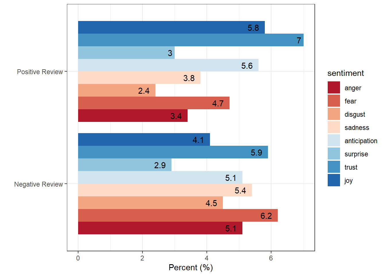
We can also visualize the results and show the rate to identify what type is more “positive” and what type is more “negative”.
reviews_summarised %>%
  dplyr::filter(sentiment != "positive",
         sentiment != "negative") %>%
  # plot
  ggplot(aes(sentiment, ratio, fill = type, label = ratio)) +
  geom_bar(stat="identity",
           position=position_fill()) +
  geom_text(position = position_fill(vjust = 0.5)) +
  scale_fill_manual(name = "", values=c("orange", "gray70")) +
  scale_y_continuous(name ="Percent", breaks = seq(0, 1, .2), labels = seq(0, 100, 20)) +
  theme_bw() +
  theme(legend.position = "top")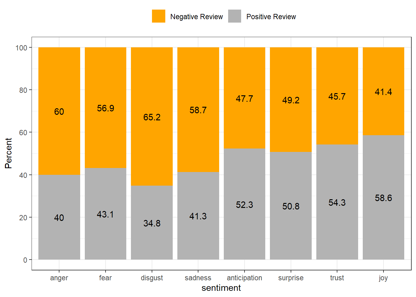
5.5 Identifying important emotives
We now check, which words have contributed to the emotionality scores. In other words, we investigate, which words are most important for the emotion scores within each review type. For the sake of interpretability, we will remove several core emotion categories and also the polarity.
# Filter the annotated reviews to exclude certain sentiments and remove NA sentiments
reviews_importance <- reviews_annotated %>%
  dplyr::filter(!is.na(sentiment),        # Keep only rows with non-NA sentiments
                sentiment != "anticipation", # Exclude 'anticipation' sentiment
                sentiment != "surprise",    # Exclude 'surprise' sentiment
                sentiment != "disgust",     # Exclude 'disgust' sentiment
                sentiment != "negative",    # Exclude 'negative' sentiment
                sentiment != "sadness",     # Exclude 'sadness' sentiment
                sentiment != "positive") %>%
  # Convert 'sentiment' to a factor with specified levels
  dplyr::mutate(sentiment = factor(sentiment, levels = c("anger", "fear", "trust", "joy"))) %>%
  # Group the data by 'type'
  dplyr::group_by(type) %>%
  # Count the occurrences of each word within each sentiment and type, sorting the counts in descending order
  dplyr::count(word, sentiment, sort = TRUE) %>%
  # Further group the data by 'type' and 'sentiment'
  dplyr::group_by(type, sentiment) %>%
  # Select the top 5 words within each 'type' and 'sentiment'
  dplyr::top_n(5) %>%
  # Calculate the score for each word as the proportion of the total count within each group
  dplyr::mutate(score = n/sum(n))
# inspect data
reviews_importance %>%
  as.data.frame() %>%
  head(10)
## type word sentiment n score
## 1 Negative Review bad anger 575 0.5203620
## 2 Negative Review bad fear 575 0.4622186
## 3 Positive Review love joy 329 0.3884298
## 4 Positive Review watch fear 296 0.4111111
## 5 Negative Review watch fear 284 0.2282958
## 6 Positive Review real trust 225 0.3040541
## 7 Negative Review pretty trust 177 0.2338177
## 8 Negative Review pretty joy 177 0.2637854
## 9 Negative Review director trust 160 0.2113606
## 10 Negative Review real trust 149 0.1968296We can now visualize the top three words for the remaining core emotion categories.
# Group the reviews importance data by 'type'
reviews_importance %>%
  dplyr::group_by(type) %>%
  # Select the top 20 rows within each group based on the 'score' column
  dplyr::slice_max(score, n = 20) %>%
  # Arrange the rows in descending order of 'score'
  dplyr::arrange(desc(score)) %>%
  # Ungroup the data to remove the grouping structure
  dplyr::ungroup() %>%
  # plot
  ggplot(aes(x = reorder(word, score), y = score, fill = word)) +
  facet_wrap(type~sentiment, ncol = 4, scales = "free_y") +
  geom_col(show.legend = FALSE) +
  coord_flip() +
  labs(x = "Words")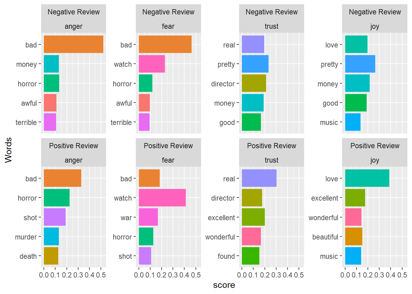
If you are interested in learning more about SA in R, Silge and Robinson (2017) is highly recommended as it goes more into detail and offers additional information.