Week 4 Getting Started with R and RStudio 1
This tutorial shows how to get started with R and it specifically focuses on R for analyzing language data but it offers valuable information for anyone who wants to get started with R. As such, this tutorial is aimed at fresh users or beginners with the aim of showcasing how to set up a R session in RStudio, how to set up R projects, and how to do basic operations using R. The aim is not to provide a fully-fledged from beginner-to-expert, all-you-need-to-know tutorial but rather to show how to properly and tidily set up a project before you start coding and exemplify common operations such as loading and manipulation tabular data and generating basic visualization using R.
If you already have experience with R, both Wickham and Grolemund (2016) (see here) and Gillespie and Lovelace (2016) (see here) are highly recommendable and excellent resources for improving your coding abilities and workflows in R.
4.1 Goals of this tutorial
The goals of this tutorial are:
- How to get started with R
- How to orient yourself to R and RStudio
- How to create and work in R projects
- How to know where to look for help and to learn more about R
- Understand the basics of working with data: load data, save data, working with tables, create a simple plot
- Learn some best practices for using R scripts, using data, and projects
- Understand the basics of objects, functions, and indexing
4.2 Audience
The intended audience for this tutorial is beginner-level, with no previous experience using R. Thus, no prior knowledge of R is required.
If you want to know more, would like to get some more practice, or would like to have another approach to R, please check out the workshops and resources on R provided by the UQ library. In addition, there are various online resources available to learn R (you can check out a very recommendable introduction here).
4.3 Installing R and RStudio
You have NOT yet installed R on your computer?
You have NOT yet installed RStudio on your computer?
- Click here for downloading and installing RStudio.
You have NOT yet downloaded the materials for this workshop?
You can find a more elaborate explanation of how to download and install R and RStudio here that was created by the UQ library.
4.3.1 How to use the workshop materials
You can follow this workshop in different ways based on your preferences as well as prior experience and knowledge of R (the suggestions listed below are ordered from less engaged/easy/no knowledge required to more engaged/more complex/more knowledge is required)
You can simply sit back and follow the workshop
You can load the Rmd-file in RStudio and execute the code snippets in this Rmd-file as we go (we will talk about what Rmd-file are, how they work, and how to work in RStudio below)
- If you decide on doing this, then I suggest, that you use a section of your screen for Zoom (to see what I do) and another section of your screen to work within your own R project (we will see what an R project is below)
You can load the Rmd-file in RStudio, create a new Rmd-file (or R Notebook) and then copy and paste the code snippets in this new Rmd-file and execute them as we go.
This option requires some knowledge of R and RStudio
If you decide on doing this, then I suggest, that you use a section of your screen for Zoom (to see what I do) and another section of your screen to work within your own R project (as with the previous option)
Future workshops will be interactive and allow you to write your own code into code boxes on the website - unfortunately, I was not able to integrate that for this workshop.
4.4 Preparation
Before you actually open R or RStudio, there things to consider that make working in R much easier and give your workflow a better structure.
Imagine it like this: when you want to write a book, you could simply take pen and paper and start writing or you could think about what you want to write about, what different chapters your book would consist of, which chapters to write first, what these chapters will deal with, etc. The same is true for R: you could simply open R and start writing code or you can prepare you session and structure what you will be doing.
4.4.1 Folder Structure and R projects
Before actually starting with writing code, you should prepare the session by going through the following steps:
4.4.2 1. Create a folder for your project
In that folder, create the following sub-folders (you can, of course, adapt this folder template to match your needs)
- data (you do not create this folder for the present workshop as you can simply use the data folder that you downloaded for this workshop instead)
- images
- tables
- docs
The folder for your project could look like the the one shown below.
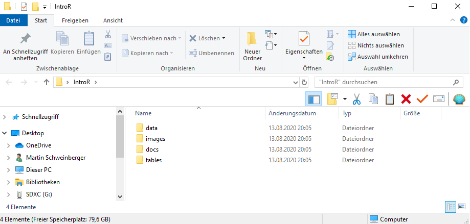
Once you have created your project folder, you can go ahead with RStudio.
4.4.3 3. Open RStudio
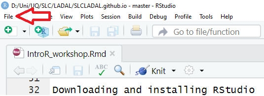
This is what RStudio looks like when you first open it:
![]()
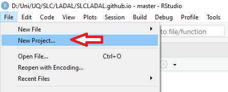
In RStudio, click on File
You can use the drop-down menu to create a R project
4.4.4 4. R Projects
In RStudio, click on New Project
Next, confirm by clicking OK and select Existing Directory.
Then, navigate to where you have just created the project folder for this workshop.
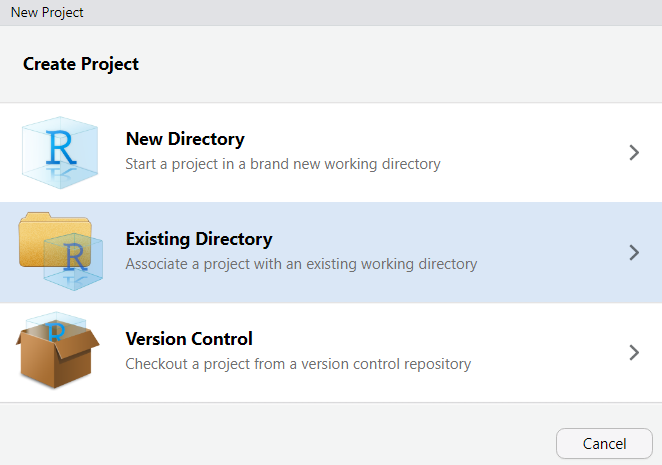
Once you click on Open, you have created a new R project
4.4.5 5. R Notebooks
In this project, click on File
Click on New File and then on R Notebook as shown below.
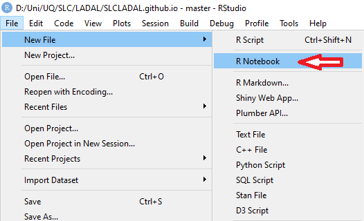
This R Notebook will be the file in which you do all your work.
4.4.6 6. Updating R
In case you encounter issues when opening the R Notebook (e.g., if you receive an error message saying that you need to update packages which then do not install properly), you may have to update your R version.
To update your current R version to the recent release please copy the code chunk shown below into the console pane (the bottom left pane) and click on Enter to run the code. The code will automatically update your version of R to the most recent release. During the update, you may be asked to specify some options - in that case, you can simply click on Accept and Next and accept the default settings.
# install installr package
install.packages("installr")
# load installr package
library(installr)
# update r
updateR()
4.4.7 7. Optimizing R project options
When you work with projects, it is recommendable to control the so-called environment. This means that you make your R Project self-contained by storing all packages that are used in project in a library in the R Project (instead of in the general R library on your computer). Having a library in your R Project means that you can share your project folder wit other people and they will automatically have the same package versions that you have sued which makes your code more robust and reproducible.
So, how to create such an environment? You simply click on Tools (at the very top right of RStudio), then click onProject Options then click on Environments and then check Use renv with this project. Now, when you install packages, they will be installed in the package library (rather than the general R library on your computer).
4.4.8 8. Getting started with R Notebooks
You can now start writing in this R Notebook. For instance, you could start by changing the title of the R Notebook and describe what you are doing (what this Notebook contains).
Below is a picture of what this document looked like when I started writing it.
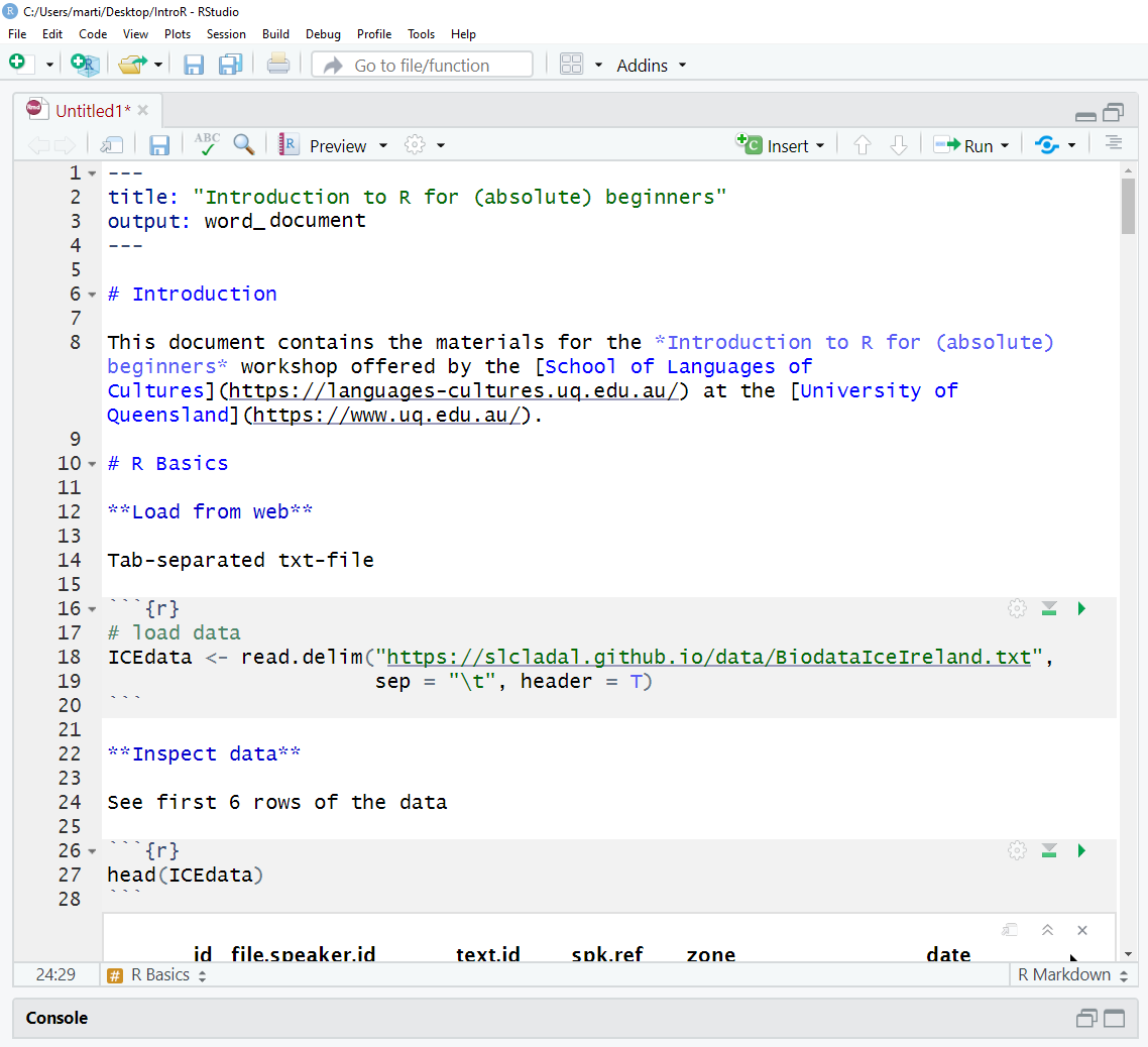
When you write in the R Notebook, you use what is called R Markdown which is explained below.
4.4.9 R Markdown
The Notebook is an R Markdown document: a Rmd (R Markdown) file is more than a flat text document: it’s a program that you can run in R and which allows you to combine prose and code, so readers can see the technical aspects of your work while reading about their interpretive significance.
You can get a nice and short overview of the formatting options in R Markdown (Rmd) files here.
R Markdown allows you to make your research fully transparent and reproducible! If a couple of years down the line another researcher or a journal editor asked you how you have done your analysis, you can simply send them the Notebook or even the entire R-project folder.
As such, Rmd files are a type of document that allows to
include snippets of code (and any outputs such as tables or graphs) in plain text while
encoding the structure of your document by using simple typographical symbols to encode formatting (rather than HTML tags or format types such as Main header or Header level 1 in Word).
Markdown is really quite simple to learn and these resources may help:
The Markdown Wikipedia page includes a very handy chart of the syntax.
John Gruber developed Markdown and his introduction to the syntax is worth browsing.
This interactive Markdown tutorial will teach you the syntax in a few minutes.
4.5 R and RStudio Basics
RStudio is a so-called IDE - Integrated Development Environment. The interface provides easy access to R. The advantage of this application is that R programs and files as well as a project directory can be managed easily. The environment is capable of editing and running program code, viewing outputs and rendering graphics. Furthermore, it is possible to view variables and data objects of an R-script directly in the interface.
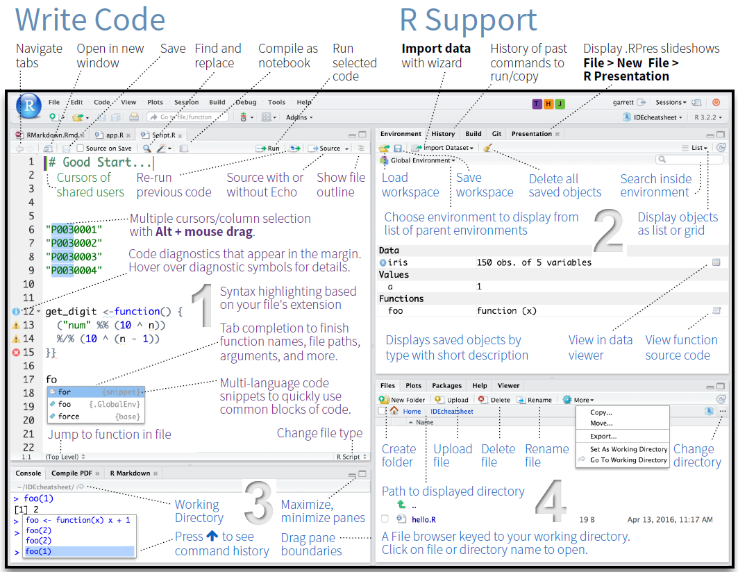
4.5.1 RStudio: Panes
The GUI - Graphical User Interface - that RStudio provides divides the screen into four areas that are called panes:
- File editor
- Environment variables
- R console
- Management panes (File browser, plots, help display and R packages).
The two most important are the R console (bottom left) and the File editor (or Script in the top left). The Environment variables and Management panes are on the right of the screen and they contain:
- Environment (top): Lists all currently defined objects and data sets
- History (top): Lists all commands recently used or associated with a project
- Plots (bottom): Graphical output goes here
- Help (bottom): Find help for R packages and functions. Don’t forget you can type
?before a function name in the console to get info in the Help section. - Files (bottom): Shows the files available to you in your working directory
These RStudio panes are shown below.
4.5.2 R Console (bottom left pane)
The console pane allows you to quickly and immediately execute R code. You can experiment with functions here, or quickly print data for viewing.
Type next to the > and press Enter to execute.
EXERCISE TIME!
`
- You can use R like a calculator. Try typing
2+8into the R console.
Answer
2+8 ## [1] 10`
Here, the plus sign is the operator. Operators are symbols that represent some sort of action. However, R is, of course, much more than a simple calculator. To use R more fully, we need to understand objects, functions, and indexing - which we will learn about as we go.
For now, think of objects as nouns and functions as verbs.
4.6 Running commands from a script
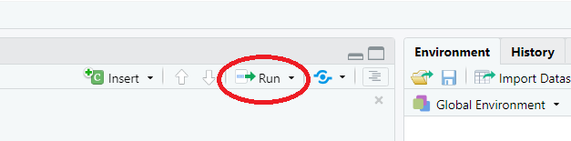
To run code from a script, insert your cursor on a line with a command, and press CTRL/CMD+Enter.
Or highlight some code to only run certain sections of the command, then press CTRL/CMD+Enter to run.
Alternatively, use the Run button at the top of the pane to execute the current line or selection (see below).
4.6.1 Script Editor (top left pane)
In contrast to the R console, which quickly runs code, the Script Editor (in the top left) does not automatically execute code. The Script Editor allows you to save the code essential to your analysis. You can re-use that code in the moment, refer back to it later, or publish it for replication.
Now, that we have explored RStudio, we are ready to get started with R!
4.7 Getting started with R
This section introduces some basic concepts and procedures that help optimize your workflow in R.
4.7.1 Setting up an R session
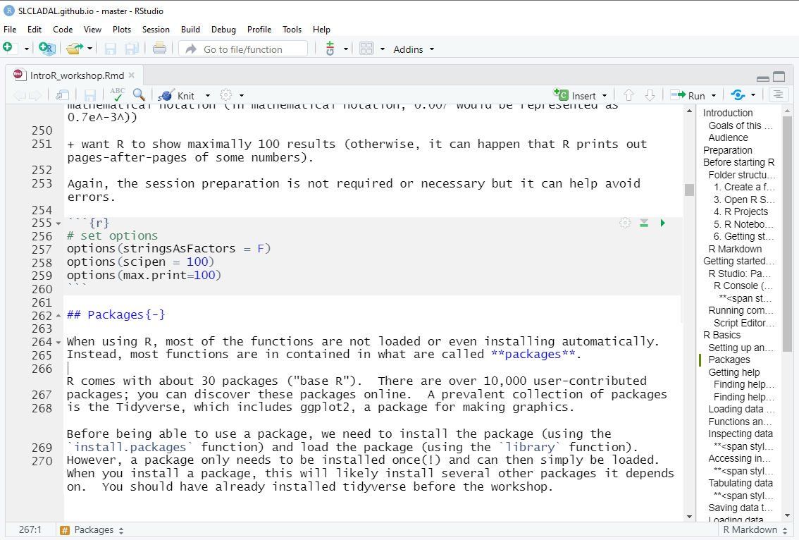
At the beginning of a session, it is common practice to define some basic parameters. This is not required or even necessary, but it may just help further down the line. This session preparation may include specifying options. In the present case, we
want R to show numbers as numbers up to 100 decimal points (and not show them in mathematical notation (in mathematical notation, 0.007 would be represented as 0.7e-3))
want R to show maximally 100 results (otherwise, it can happen that R prints out pages-after-pages of some numbers).
Again, the session preparation is not required or necessary but it can help avoid errors.
# set options
options(stringsAsFactors = F)
options(scipen = 100)
options(max.print=100)
In script editor pane of RStudio, this would look like this:
4.7.2 Packages
When using R, most of the functions are not loaded or even installing automatically. Instead, most functions are in contained in what are called packages.
R comes with about 30 packages (“base R”). There are over 10,000 user-contributed packages; you can discover these packages online. A prevalent collection of packages is the Tidyverse, which includes ggplot2, a package for making graphics.
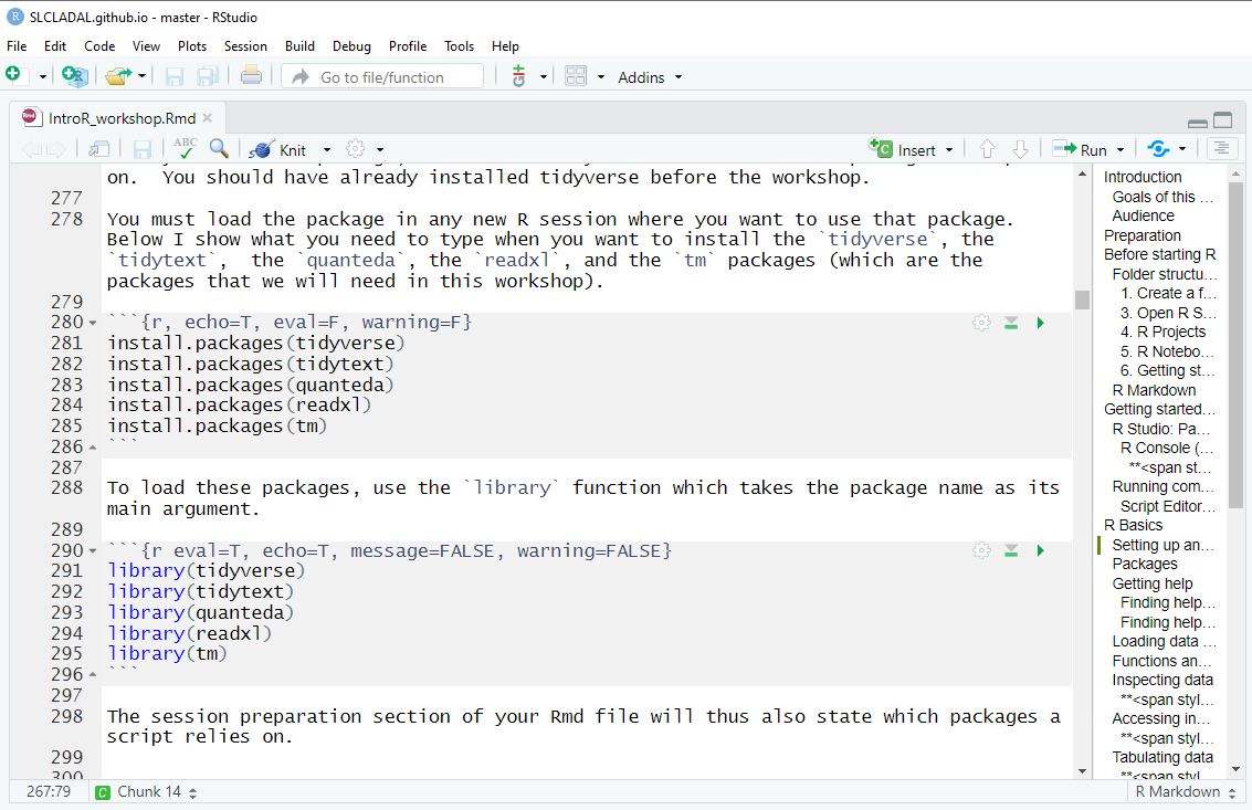
Before being able to use a package, we need to install the package (using the install.packages function) and load the package (using the library function). However, a package only needs to be installed once(!) and can then simply be loaded. When you install a package, this will likely install several other packages it depends on. You should have already installed tidyverse before the workshop.
You must load the package in any new R session where you want to use that package. Below I show what you need to type when you want to install the tidyverse, the tidytext, the quanteda, the readxl, and the tm packages (which are the packages that we will need in this workshop).
install.packages("tidyverse")
install.packages("tidytext")
install.packages("quanteda")
install.packages("readxl")
install.packages("tm")
install.packages("tokenizers")
install.packages("here")
install.packages("flextable")
# install klippy for copy-to-clipboard button in code chunks
install.packages("remotes")
remotes::install_github("rlesur/klippy")
To load these packages, use the library function which takes the package name as its main argument.
library(tidyverse)
library(tidytext)
library(quanteda)
library(readxl)
library(tm)
library(tokenizers)
library(here)
library(flextable)
# activate klippy for copy-to-clipboard button
klippy::klippy()
The session preparation section of your Rmd file will thus also state which packages a script relies on.
In script editor pane of RStudio, the code blocks that install and activate packages would look like this:
4.7.3 Getting help
When working with R, you will encounter issues and face challenges. A very good thing about R is that it provides various ways to get help or find information about the issues you face.
4.7.3.1 Finding help within R
To get help regrading what functions a package contains, which arguments a function takes or to get information about how to use a function, you can use the help function or the apropos. function or you can simply type a ? before the package or two ?? if this does not give you any answers.
help(tidyverse)
apropos("tidyverse")
?require
There are also other “official” help resources from R/RStudio.
Read official package documentation, see vignettes, e.g., Tidyverse https://cran.r-project.org/package=tidyverse
Use the RStudio Cheat Sheets at https://www.rstudio.com/resources/cheatsheets/
Use the RStudio Help viewer by typing
?before a function or packageCheck out the keyboard shortcuts
HelpunderToolsin RStudio for some good tips
4.7.3.2 Finding help online
One great thing about R is that you can very often find an answer to your question online.
- Google your error! See http://r4ds.had.co.nz/introduction.html#getting-help-and-learning-more for excellent suggestions on how to find help for a specific question online.
4.8 Working with tables
We will now start working with data in R. As most of the data that we work with comes in tables, we will focus on this first before moving on to working with text data.
4.8.1 Loading data from the web
To show, how data can be downloaded from the web, we will download a tab-separated txt-file. Translated to prose, the code below means Create an object called icebio and in that object, store the result of the read.delim function.
read.delim stands for read delimited file and it takes the URL from which to load the data (or the path to the data on your computer) as its first argument. The sep stand for separator and the \t stands for tab-separated and represents the second argument that the read.delim function takes. The third argument, header, can take either T(RUE) or F(ALSE) and it tells R if the data has column names (headers) or not.
4.8.2 Functions and Objects
In R, functions always have the following form: function(argument1, argument2, ..., argumentN). Typically a function does something to an object (e.g. a table), so that the first argument typically specifies the data to which the function is applied. Other arguments then allow to add some information. Just as a side note, functions are also objects that do not contain data but instructions.
To assign content to an object, we use <- or = so that the we provide a name for an object, and then assign some content to it. For example, MyObject <- 1:3 means Create an object called MyObject. this object should contain the numbers 1 to 3.
# load data
icebio <- read.delim("https://slcladal.github.io/data/BiodataIceIreland.txt",
                      sep = "\t", header = T)
4.8.3 Inspecting data
There are many ways to inspect data. We will briefly go over the most common ways to inspect data.
The head function takes the data-object as its first argument and automatically shows the first 6 elements of an object (or rows if the data-object has a table format).
head(icebio)## id file.speaker.id text.id spk.ref zone date sex age
## 1 1 <S1A-001$A> S1A-001 A northern ireland 1990-1994 male 34-41
## 2 2 <S1A-001$B> S1A-001 B northern ireland 1990-1994 female 34-41
## 3 3 <S1A-002$?> S1A-002 ? <NA> <NA> <NA> <NA>
## 4 4 <S1A-002$A> S1A-002 A northern ireland 2002-2005 female 26-33
## 5 5 <S1A-002$B> S1A-002 B northern ireland 2002-2005 female 19-25
## 6 6 <S1A-002$C> S1A-002 C northern ireland 2002-2005 male 50+
## word.count
## 1 765
## 2 1298
## 3 23
## 4 391
## 5 47
## 6 200We can also use the head function to inspect more or less elements and we can specify the number of elements (or rows) that we want to inspect as a second argument. In the example below, the 4 tells R that we only want to see the first 4 rows of the data.
head(icebio, 4)## id file.speaker.id text.id spk.ref zone date sex age
## 1 1 <S1A-001$A> S1A-001 A northern ireland 1990-1994 male 34-41
## 2 2 <S1A-001$B> S1A-001 B northern ireland 1990-1994 female 34-41
## 3 3 <S1A-002$?> S1A-002 ? <NA> <NA> <NA> <NA>
## 4 4 <S1A-002$A> S1A-002 A northern ireland 2002-2005 female 26-33
## word.count
## 1 765
## 2 1298
## 3 23
## 4 391EXERCISE TIME!
`
- Download and inspect the first 7 rows of the data set that you can find under this URL:
https://slcladal.github.io/data/lmmdata.txt. Can you guess what the data is about?
Answer
  ex1data <- read.delim("https://slcladal.github.io/data/lmmdata.txt", sep = "\t")
  head(ex1data, 7)
## Date Genre Text Prepositions Region
## 1 1736 Science albin 166.01 North
## 2 1711 Education anon 139.86 North
## 3 1808 PrivateLetter austen 130.78 North
## 4 1878 Education bain 151.29 North
## 5 1743 Education barclay 145.72 North
## 6 1908 Education benson 120.77 North
## 7 1906 Diary benson 119.17 NorthDate), the genre the texts represent (Genre), the name of the texts (Text), the relative frequencies of prepositions the texts contain (Prepositions), and the region where the author was from (Region).
`
4.8.4 Accessing individual cells in a table
If you want to access specific cells in a table, you can do so by typing the name of the object and then specify the rows and columns in square brackets (i.e. data[row, column]). For example, icebio[2, 4] would show the value of the cell in the second row and fourth column of the object icebio. We can also use the colon to define a range (as shown below, where 1:5 means from 1 to 5 and 1:3 means from 1 to 3) The command icebio[1:5, 1:3] thus means:
Show me the first 5 rows and the first 3 columns of the data-object that is called icebio.
icebio[1:5, 1:3]## id file.speaker.id text.id
## 1 1 <S1A-001$A> S1A-001
## 2 2 <S1A-001$B> S1A-001
## 3 3 <S1A-002$?> S1A-002
## 4 4 <S1A-002$A> S1A-002
## 5 5 <S1A-002$B> S1A-002EXERCISE TIME!
`
- How would you inspect the content of the cells in 4th column, rows 3 to 5 of the
icebiodata set?
Answer
icebio[3:5, 4] ## [1] "?" "A" "B"`
Inspecting the structure of data
You can use the str function to inspect the structure of a data set. This means that this function will show the number of observations (rows) and variables (columns) and tell you what type of variables the data consists of
- int = integer
- chr = character string
- num = numeric
- fct = factor
str(icebio)## 'data.frame': 1332 obs. of 9 variables:
## $ id : int 1 2 3 4 5 6 7 8 9 10 ...
## $ file.speaker.id: chr "<S1A-001$A>" "<S1A-001$B>" "<S1A-002$?>" "<S1A-002$A>" ...
## $ text.id : chr "S1A-001" "S1A-001" "S1A-002" "S1A-002" ...
## $ spk.ref : chr "A" "B" "?" "A" ...
## $ zone : chr "northern ireland" "northern ireland" NA "northern ireland" ...
## $ date : chr "1990-1994" "1990-1994" NA "2002-2005" ...
## $ sex : chr "male" "female" NA "female" ...
## $ age : chr "34-41" "34-41" NA "26-33" ...
## $ word.count : int 765 1298 23 391 47 200 464 639 308 78 ...The summary function summarizes the data.
summary(icebio)## id file.speaker.id text.id spk.ref
## Min. : 1.0 Length:1332 Length:1332 Length:1332
## 1st Qu.: 333.8 Class :character Class :character Class :character
## Median : 666.5 Mode :character Mode :character Mode :character
## Mean : 666.5
## 3rd Qu.: 999.2
## Max. :1332.0
## zone date sex age
## Length:1332 Length:1332 Length:1332 Length:1332
## Class :character Class :character Class :character Class :character
## Mode :character Mode :character Mode :character Mode :character
##
##
##
## word.count
## Min. : 0.0
## 1st Qu.: 66.0
## Median : 240.5
## Mean : 449.9
## 3rd Qu.: 638.2
## Max. :2565.0