Week 13 Tree-Based Models
This week, we focus on tree-based models and their implementation in R.
The Basic Concept
This section deals with tree-structure models which fall into the machine-learning rather than the inference statistics category as they are commonly used for classification and prediction tasks rather than explanation of relationships between variables. This means that tree-based models are typically used in classification tasks rather than in inferential analyses where we want to see how strongly factors of interactions between factors impact an outcome.
The most basic type of tree-structure model is a decision tree or CART (classification and regression tree). A more optimized version of CARTs are conditional inference trees (CITs) - although CART and CITs are commonly treated as one and the same thing although CITs differ from CARTs in that they provide more accurate variable importance measures. Like random forests, inference trees are non-parametric and thus do not rely on distributional requirements (or at least on fewer). The tree structure represents recursive partitioning of the data to minimize residual deviance.
CARTs consist of three parts: a root, nodes, and leaves.
- The root is the first split in a CART - if there is not split, then the root is also a leave (an endpoint)
- Leaves form the endpoint of paths and represent the outcome of a classification (or decision)
- Nodes represent the path and reflect the partitioning of the data. At each node the data is split and the node has two outgoing paths to the subsets of the data.
Advantages of tree-based models
Over the past 10 or so years, tree-based models have become really popular in applied linguistics and related fields. This is because such models have (or are assumed to have) the following advantages:
Tree-structure models are very useful because they can deal with different types of variables and provide a very good understanding of the structure in the data.
Tree-structure models have been deemed particularly interesting for linguists because they can handle moderate sample sizes and many high-order interactions better then regression models.
Tree-structure models are (supposedly) better at detecting non-linear or non-monotonic relationships between predictors and dependent variables.
Tree-structure models are easy to implement in R and do not require the model selection, validation, and diagnostics associated with regression models.
Tree-structure models can be used as variable-selection procedure which informs about which variables have any sort of significant relationship with the dependent variable and can thereby inform model fitting.
Problems of tree-based models
Despite these potential advantages, a word of warning is in order: Gries (2021) admits that tree-based models can be very useful but that they can suffer from issues which can lead to some serious short-comings which remain under-explored. For instance,
Tree-structure models do not reflect or model nested or hierarchical data structures (unlike mixed-effects models). This is a major disadvantage as most data in applied linguistics is nested in some form.
Tree-structure models do not provide effect sizes for main effects and interactions but only inform about the overall importance of a variable or its importance within subsets of the data. Thus, tree-structure models do not show how important a variable is by itself. When dealing with Random Forest or Boruta, we also do not know is a variable is important as a main effect or as part of interactions (or both)! The importance only shows that there is some important connection between the predictor and the dependent variable.
Simple tree-structure models have been shown to fail in detecting the correct predictors if the variance is solely determined by a single interaction (Gries 2021, chap. 7.3). This failure is caused by the fact that the predictor used in the first split of a tree is selected as the one with the strongest main effect (Boulesteix et al. 2015, 344). This issue can, however, be avoided by hard-coding the interactions as predictors plus using ensemble methods such as random forests rather than individual trees.
Another shortcoming is that tree-structure models partition the data (rather than “fitting a line” through the data which can lead to more coarse-grained predictions compared to regression models when dealing with numeric dependent variables (again, see Gries 2021, chap. 7.3).
Boulesteix et al. (2015, 341) state that high correlations between predictors can hinder the detection of interactions when using small data sets. However, regression do not fare better here as they are even more strongly affected by (multi-)collinearity.
Tree-structure models are bad a detecting interactions when the variables have strong main effects which is, unfortunately, common when dealing with linguistic data.
Before we implement a conditional inference tree in R, we will have a look at how decision trees work. We will do this in more detail here as random forests and Boruta analyses are extensions of inference trees and are therefore based on the same concepts.
13.1 Decision Trees
The most basic type of tree-structure model is a decision tree which is a type of classification and regression tree (CART). A more elaborate version of a CART is called a Conditional Inference Tree (CIT). The difference between a CART and a CIT is that CITs use significance tests, e.g. the p-values, to select and split variables rather than some information measures like the Gini coefficient (Gries 2021). Let us now see how we can generate a decision tree.
Preparation and session set up
For this week, we need to install certain packages from an R library so that the scripts shown below are executed without errors. Before turning to the code below, please install the packages by running the code below this paragraph.
# install packages
install.packages("dplyr")
install.packages("party")
install.packages("partykit")
install.packages("flextable")
Now that we have installed the packages, we can activate them as shown below.
# set options
options(scipen = 999)
# load packages
library(dplyr)
library(party)
library(partykit)
library(flextable)
We can now load and inspect the data.
# load data
citdata <- read.delim("https://slcladal.github.io/data/treedata.txt", header = T, sep = "\t")  %>%
  # convert character strings to factors
dplyr::mutate_if(is.character, factor)Age | Gender | Status | LikeUser |
15-40 | female | high | no |
15-40 | female | high | no |
15-40 | male | high | no |
41-80 | female | low | yes |
41-80 | male | high | no |
41-80 | male | low | no |
41-80 | female | low | yes |
15-40 | male | high | no |
41-80 | male | low | no |
41-80 | male | low | no |
Next, we generate and plot the decision tree.
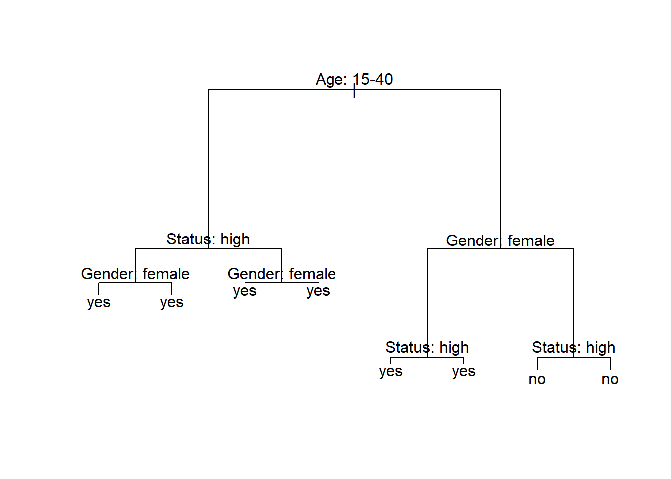
The example of the decision tree above shows what what response to expect - in this case whether a speaker uses discourse like or not. Decision trees, like all CARTs and CITs, answer a simple question, namely How do we best classify elements based on the given predictors?. The answer that decision trees provide is the classification of the elements based on the levels of the predictors.
In simple decision trees, all predictors, even those that are not significant are included in the decision tree. The decision tree shows that the best (or most important) predictor for the use of discourse like is the age of speakers as it is the highest node. Among young speakers, those with high status use like more compared with speakers of lower social status. Among old speakers, women use discourse like more than men.
The yes and no at the bottom show if the speaker should be classified as a user of discourse like (yes or no). Each split can be read as true to the left and false to the right. So that, at the first split, if the person is between the ages of 15 and 40, we need to follow the branch to the left while we need to follow to the right if the person is not 15 to 40.
Let us go over some basic concepts. The top of the decision tree is called root or root node, the categories at the end of branches are called leaves or leaf nodes. Nodes that are in-between the root and leaves are called internal nodes or just nodes. The root node has only arrows or lines pointing away from it, internal nodes have lines going to and from them, while leaf nodes only have lines pointing towards them.
13.2 Conditional Inference Trees
We now focus on Conditional Inference Trees (CITs). In contrast to decision trees, which indicate an outcome for all possible decisions, CITs only split the data if the split is statistically justified (this mean that splits are based on significant differences in the distributions resulting from the split).
Conditional Inference Trees (CITs) are much better at determining the true effect of a predictor, i.e. the effect of a predictor if all other effects are simultaneously considered. In contrast to CARTs, CITs typically use p-values to determine splits in the data. Below is a conditional inference tree which shows how and what factors contribute to the use of discourse like. In conditional inference trees predictors are only included if the predictor is significant (i.e. if these predictors are necessary).
# create initial conditional inference tree model
citd.ctree <- partykit::ctree(LikeUser ~ Age + Gender + Status, data = citdata)
# plot final ctree
plot(citd.ctree, gp = gpar(fontsize = 8)) 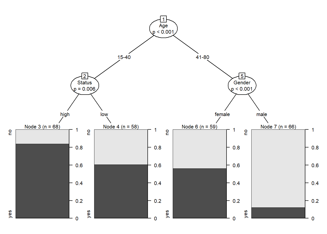
Problems of Conditional Inference Trees
Like other tree-based methods, CITs are very intuitive, multivariate, non-parametric, they do not require large data sets, and they are easy to implement. Despite these obvious advantages, they have at least one major short coming compared to other, more sophisticated tree-structure models (in addition to the general issues that tree-structure models exhibit as discussed above):
they are prone to overfitting which means that they fit the observed data very well but preform much worse when being applied to new data.
they have a strong bias towards variables with many levels, e.g., numeric variables (but also categorical variables with many levels), and they overestimate the importance of such variables.
An extension which remedies this problem is to use a so-called ensemble method which grows many varied trees. The most common ensemble method is called a Random Forest Analysis and an even better ensemble method is called Boruta (but we will not discuss them in this section - a tutorial covering these methods can be found here).