Part 6 Optimizing R Workflows

While most researchers in the language sciences are somewhat familiar with R, workshops focusing on specific tasks, such as statistical analyses in R, are increasingly common. However, workshops dedicated to general proficiency in R are rare.

When discussing ‘working in R,’ I refer to concerns surrounding reproducible and efficient workflows, session management, and adherence to formatting conventions for R code. The subsequent sections will offer guidance on optimizing workflows and enhancing research practices to foster transparency, efficiency, and reproducibility.

Rproj

If you’re utilizing RStudio, you can create a new R project, which is essentially a working directory identified by a .RProj file. When you open a project (either through ‘File/Open Project’ in RStudio or by double-clicking on the .RProj file outside of R), the working directory is automatically set to the location of the .RProj file.

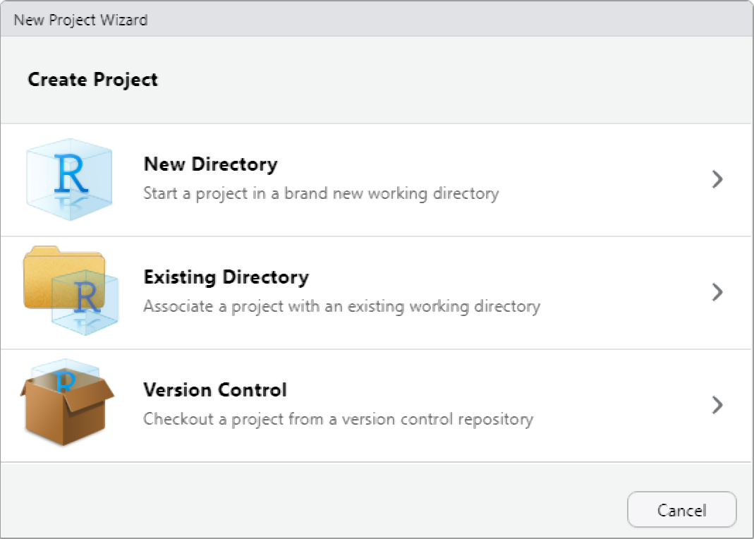
I highly recommend creating a new R Project at the outset of each research endeavor. Upon creating a new R project, promptly organize your directory by establishing folders to house your R code, data files, notes, and other project-related materials. This can be done outside of R on your computer or within the Files window of RStudio. For instance, consider creating a ‘R’ folder for your R code and a ‘data’ folder for your datasets.

Prior to adopting R Projects, I used setwd() to set my working directory. However, this method has drawbacks as it requires specifying an absolute file path, which can lead to broken scripts and hinder collaboration and reproducibility efforts. Consequently, reliance on setwd() impedes the sharing and transparency of analyses and projects. By contrast, utilizing R Projects streamlines workflow management and facilitates reproducibility and collaboration.

Dependency Control (renv)

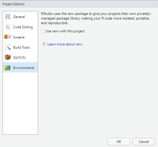
The renv package introduces a novel approach to enhancing the independence of R projects by eliminating external dependencies. By creating a dedicated library within your project, renv ensures that your R project operates autonomously from your personal library. Consequently, when sharing your project, the associated packages are automatically included.

renv aims to provide a robust and stable alternative to the packrat package, which, in my experience, fell short of expectations. Having utilized renv myself, I found it to be user-friendly and reliable. Although the initial generation of the local library may require some time, it seamlessly integrates into workflows without causing any disruptions. Overall, renv is highly recommended for simplifying the sharing of R projects, thereby enhancing transparency and reproducibility.

One of renv’s core principles is to preserve existing workflows, ensuring that they function as before while effectively isolating the R dependencies of your project, including package versioning.

For more information on renv and its functionalities, as well as guidance on its implementation, refer to the official documentation.

Version Control with Git

Getting started with Git

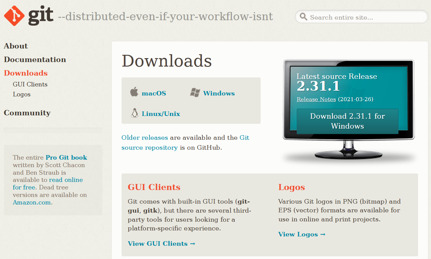
To connect your Rproject with GitHub, you need to have Git installed (if you have not yet downloaded and installed Git, simply search for download git in your favorite search engine and follow the instructions) and you need to have a GitHub account. If you do not have a GitHub account, here is a video tutorial showing how you can do this. If you have trouble with this, you can also check out Happy Git and GitHub for the useR at happygitwithr.com.

Just as a word of warning: when I set up my connection to Git and GitHUb things worked very differently, so things may be a bit different on your machine. In any case, I highly recommend this YouTube tutorial which shows how to connect to Git and GitHub using the usethis package or this, slightly older, YouTube tutorial on how to get going with Git and GitHub when working with RStudio.

Old school

While many people use the usethis package to connect RStudio to GitHub, I still use a somewhat old school way to connect my projects with GitHub. I have decided to show you how to connect RStudio to GitHub using this method, as I actually think it is easier once you have installed Git and created a gitHub account.

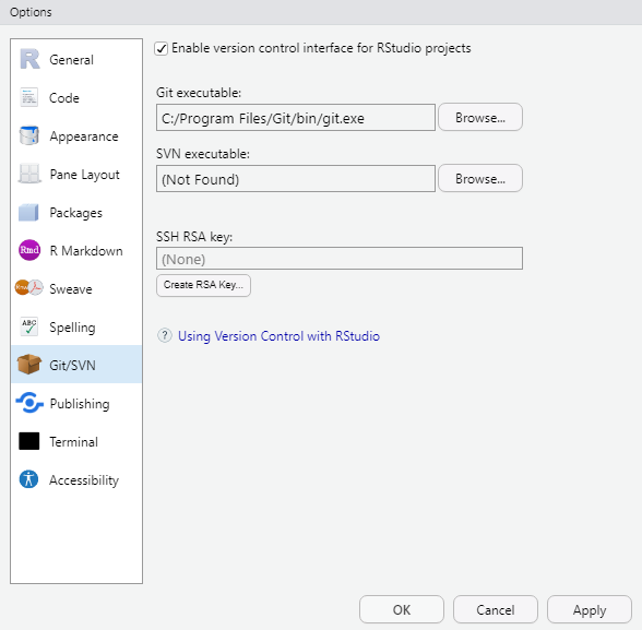
Before you can use Git with R, you need to tell RStudio that you want to use Git. To do this, go to Tools, then Global Options and then to Git/SVN and make sure that the box labeled Enable version control interface for RStudio projects. is checked. You need to then browse to the Git executable file (for Window’s users this is called the Git.exe file).

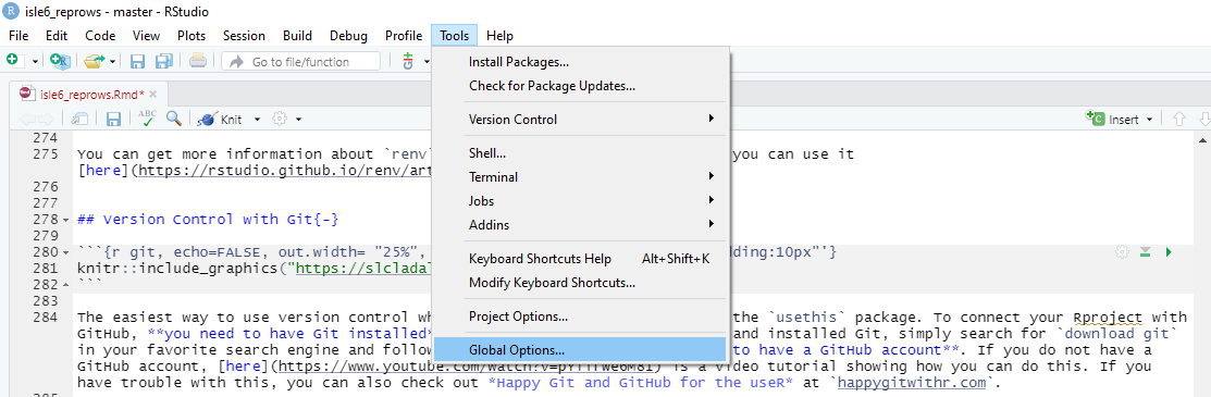
Now, we can connect our project to Git (not to GitHub yet). To do this, go to Tools, then to Project Options... and in the Git/SVN tab, change Version Control System to Git (from None). Once you have accepted these changes, a new tab called Git appears in the upper right pane of RStudio (you may need to / be asked to restart RStudio at this point). You can now commit files and changes in files to Git.

To commit files, go to the Git tab and check the boxes next to the files you would like to commit (this is called staging; meaning that these files are now ready to be committed). Then, click on Commit and enter a message in the pop-up window that appears. Finally, click on the commit button under the message window.

Connecting your Rproj with GitHub

To integrate your R project with GitHub, start by navigating to your GitHub page and create a new repository (repo). You can name it anything you like; for instance, let’s call it test. To create a new repository on GitHub, simply click on the New icon and then select New Repository. While creating the repository, I recommend checking the option to ‘Add a README’, where you can provide a brief description of the contents, although it’s not mandatory.

Once you’ve created the GitHub repo, the next step is to connect it to your local computer. This is achieved by ‘cloning’ the repository. Click on the green Code icon on your GitHub repository page, and from the dropdown menu that appears, copy the URL provided under the clone with HTTPS section.

Now, open your terminal (located between Console and Jobs in RStudio) and navigate to the directory where you want to store your project files. Use the cd command to change directories if needed. Once you’re in the correct directory, include the URL you copied from the git repository after the command git remote add origin. This sets up the connection between your local directory and the GitHub repository.

Next, execute the command git branch -M main to rename the default branch to main. This step is necessary to align with recent changes in GitHub’s naming conventions, merging the previous master and main branches.

Finally, push your local files to the remote GitHub repository by using the command git push -u origin main. This command uploads your files to GitHub, making them accessible to collaborators and ensuring version control for your project.

Following these steps ensures seamless integration between your R project and GitHub, facilitating collaboration, version control, and project management.

# initiate the upstream tracking of the project on the GitHub repo
git remote add origin https://github.com/YourGitHUbUserName/YouGitHubRepositoryName.git
# set main as main branch (rather than master)
git branch -M main
# push content to main
git push -u origin main

We can then commit changes and push them to the remote GitHub repo.

You can then go to your GitHub repo and check if the documents that we pushed are now in the remote repo.

From now on, you can simply commit all changes that you make to the GitHub repo associated with that Rproject. Other projects can, of course, be connected and push to other GitHub repos.

Solving path issues: here

The primary objective of the here package is to streamline file referencing within project-oriented workflows. Unlike the conventional approach of using setwd(), which is susceptible to fragility and heavily reliant on file organization, here leverages the top-level directory of a project to construct file paths effortlessly.

This approach significantly enhances the robustness of your projects, ensuring that file paths remain functional even if the project is relocated or accessed from a different computer. Moreover, the here package mitigates compatibility issues when transitioning between different operating systems, such as Mac and Windows, which traditionally require distinct path specifications.

# define path
example_path_full <- "D:\\Uni\\Konferenzen\\ISLE\\ISLE_2021\\isle6_reprows/repro.Rmd"
# show path
example_path_full

## [1] "D:\\Uni\\Konferenzen\\ISLE\\ISLE_2021\\isle6_reprows/repro.Rmd"

With the here package, the path starts in folder where the Rproj file is. As the Rmd file is in the same folder, we only need to specify the Rmd file and the here package will add the rest.

# load package
library(here)
# define path using here
example_path_here <- here::here("repro.Rmd")
#show path
example_path_here

## [1] "C:/Users/uqmschw5/OneDrive - The University of Queensland/Desktop/ReproALS2024/repro.Rmd"

Reproducible randomness: set.seed

The set.seed function in R sets the seed of R‘s random number generator, which is useful for creating simulations or random objects that can be reproduced. This means that when you call a function that uses some form of randomness (e.g. when using random forests), using the set.seed function allows you to replicate results.

Below is an example of what I mean. First, we generate a random sample from a vector.

numbers <- 1:10
randomnumbers1 <- sample(numbers, 10)
randomnumbers1

##  [1]  8  4  3  6  7  5  1 10  9  2

We now draw another random sample using the same sample call.

randomnumbers2 <- sample(numbers, 10)
randomnumbers2

##  [1]  2  8  6  3  5  1  7  9 10  4

As you can see, we now have a different string of numbers although we used the same call. However, when we set the seed and then generate a string of numbers as show below, we create a reproducible random sample.

set.seed(123)
randomnumbers3 <- sample(numbers, 10)
randomnumbers3

##  [1]  3 10  2  8  6  9  1  7  5  4

To show that we can reproduce this sample, we call the same seed and then generate another random sample which will be the same as the previous one because we have set the seed.

set.seed(123)
randomnumbers4 <- sample(numbers, 10)
randomnumbers4

##  [1]  3 10  2  8  6  9  1  7  5  4

Tidy data principles

The same (underlying) data can be represented in multiple ways. The following three tables are show the same data but in different ways.

Table 6.1: Table 6.2: Table 1.
country	continent	2002	2007
Afghanistan	Asia	42.129	43.828
Australia	Oceania	80.370	81.235
China	Asia	72.028	72.961
Germany	Europe	78.670	79.406
Tanzania	Africa	49.651	52.517

Table 6.3: Table 6.4: Table 2.
year	Afghanistan (Asia)	Australia (Oceania)	China (Asia)	Germany (Europe)	Tanzania (Africa)
2002	42.129	80.370	72.028	78.670	49.651
2007	43.828	81.235	72.961	79.406	52.517

Table 6.5: Table 6.6: Table 3.
country	year	continent	lifeExp
Afghanistan	2002	Asia	42.129
Afghanistan	2007	Asia	43.828
Australia	2002	Oceania	80.370
Australia	2007	Oceania	81.235
China	2002	Asia	72.028
China	2007	Asia	72.961
Germany	2002	Europe	78.670
Germany	2007	Europe	79.406
Tanzania	2002	Africa	49.651
Tanzania	2007	Africa	52.517

Table 3 should be the easiest to parse and understand. This is so because only Table 3 is tidy. Unfortunately, however, most data that you will encounter will be untidy. There are two main reasons:

Most people aren’t familiar with the principles of tidy data, and it’s hard to derive them yourself unless you spend a lot of time working with data.
Data is often organised to facilitate some use other than analysis. For example, data is often organised to make entry as easy as possible.

This means that for most real analyses, you’ll need to do some tidying. The first step is always to figure out what the variables and observations are. Sometimes this is easy; other times you’ll need to consult with the people who originally generated the data. The second step is to resolve one of two common problems:

One variable might be spread across multiple columns.
One observation might be scattered across multiple rows.

To avoid structuring in ways that make it harder to parse, there are three interrelated principles which make a data set tidy:

Each variable must have its own column.
Each observation must have its own row.
Each value must have its own cell.

An additional advantage of tidy data is that is can be transformed more easily into any other format when needed.

How to minimize storage space

Most people use or rely on data that comes in spreadsheets and use software such as Microsoft Excel or OpenOffice Calc. However, spreadsheets produced by these software applications take up a lot of storage space.

One way to minimize the space, that your data takes up, is to copy the data and paste it into a simple editor or txt-file. The good thing about txt files is that they take up only very little space and they can be viewed easily so that you can open the file to see what the data looks like. You could then delete the spread sheet because you can copy and paste the content of the txt file right back into a spread sheet when you need it.

If you work with R, you may also consider to save your data as .rda files which is a very efficient way to save and story data in an R environment

Below is an example for how you can load, process, and save your data as .rda in RStudio.

# load data
lmm <- read.delim("https://slcladal.github.io/data/lmmdata.txt", header = TRUE)
# convert strings to factors
lmm <- lmm %>%
  dplyr::mutate(Genre = factor(Genre),
                Text = factor(Text),
                Region = factor(Region))
# save data
base::saveRDS(lmm, file = here::here("data", "lmm_out.rda"))
# remove lmm object
rm(lmm)
# load .rda data
lmm  <- base::readRDS(file = here::here("data", "lmm_out.rda"))
# or from web
lmm  <- base::readRDS(url("https://slcladal.github.io/data/lmm.rda", "rb"))
# inspect data
str(lmm)

## 'data.frame':    537 obs. of  5 variables:
##  $ Date        : int  1736 1711 1808 1878 1743 1908 1906 1897 1785 1776 ...
##  $ Genre       : Factor w/ 16 levels "Bible","Biography",..: 13 4 10 4 4 4 3 9 9 3 ...
##  $ Text        : Factor w/ 271 levels "abott","albin",..: 2 6 12 16 17 20 20 24 26 27 ...
##  $ Prepositions: num  166 140 131 151 146 ...
##  $ Region      : Factor w/ 2 levels "North","South": 1 1 1 1 1 1 1 1 1 1 ...

To compare, the lmmdata.txt requires 19.2KB while the lmmdata.rda only requires 5.2KB (and only 4.1KB with xz compression). If stored as an Excel spreadsheet, the same file requires 28.6KB.